Electromagnetic Radiation, RF Pulses and Radar
A radar transmitter generates multiple forms of electromagnetic energy. This energy is amplified and transmitted and ultimately is reflected off a target, received and the difference in time and frequency of the transmit signal verses the received signal is used to determine the distance and velocity of a target.
Referring to figure 1; a pulse of energy is generated at an instance in time (ttx) with a specific power (Ptx), and frequency (ftransmit) and the energy is radiated using an antenna with gain (G). The energy propagates through the air at the speed of light (C). A target with an electromagnetic cross section (theta) will absorb some of the energy and reflect a portion the energy back to a receiver (Scattering), which in many cases is co-locate with the transmitter. The time it takes for the round trip of energy is the difference in time between the received energy and the transmitted energy multiplied by the speed of light. As we are interested in the distance of the target, we divide the round trip time by two. If the target is moving there will also be a slight frequency shift by also comparing the transmit frequency to the received frequency, we can determine the targets velocity and determine if it is getting closer to the transmitter or moving away.
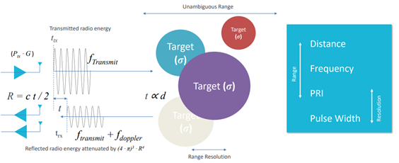 Figure 1
A radar constantly repeats the above process multiple times, if the repetition time, or Pulse Repletion Interval (PRI) is low, or if the pulse on-time - Pulse Width (PW) is long then the Radars ability to distinguish two or more close together targets is diminished, this is referred to as ambiguous operation. However, as we will learn short pulses, high PRI’s and High Frequencies cannot propagate through free space as easily as low frequencies, so a Radar will always be making a tradeoff between Resolution and Range. In some cases, a system will have multiple radars, one with low frequencies and long duration energy pulses to look for targets at distance (Search Radar), and a second that can rapidly change the pulse repetition interval and pulse types to be able to identify targets at close range with high resolution and the least ambiguity (Track and Fire Control Radar).
Calculating Radar Range
How RF energy propagates in a Radar system is modeled using the Radar Range Equation. Consider the following equation.
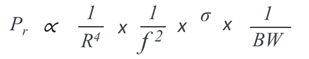
The receiver power is proportional to the reciprocal of distance R to the power of 4. Why? We assume that that the target is spherical and that we illuminate a small cross section, so the power of 4 is derived from the calculation of spherical area. As you can see the power diminishes rapidly as the target distance increases – this is the biggest loss in the system. The received power is further decreased by the reciprocal of the frequency squared. Then again by how much of the energy is absorbed or reflected (scattered), then finally by the reciprocal of the Bandwidth off the signal.
We can break the above equation down into the following blocks, The combined energy of the transmitter power and antenna gain R meters from the transmitter radiated on a sphere, the scattered energy reflected from the target, the gain of the received antenna. At this point the received signal is very low compared to the transmit signal so we must consider the low noise capability of the receiver, which deteriorates with wider bandwidth and higher frequencies.
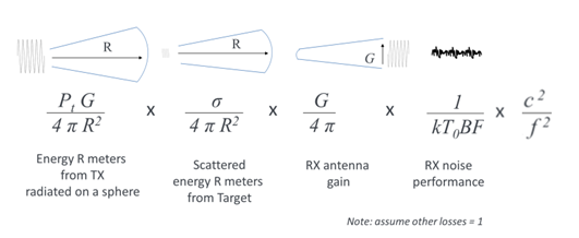
As you can see, we have more losses than gains in the system. At this point it is worth examining the antenna systems and the power amplifier. An antenna is a passive device, so how can it have gain. It doesn’t amplify the signal in reality but focuses the radiation in one direction. For example, (Figure 2) an isotropic antenna radiates energy equally in all directions, compared to a directional antenna such as a Yagi antenna sums all the isotropic energy and focuses it on one direction. Thus, using a directional antenna, we effectively add some gain to the system.
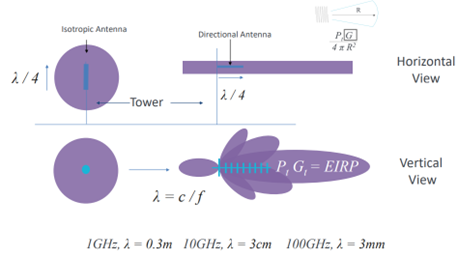 Figure 2
Our range equation says that the range decreases with higher frequencies (1/f), so lower frequencies will propagate further. Also note that the frequency defines the size of the antenna. Wavelength decreases in value as the transmit frequency gets higher. So low frequency systems, i.e., systems optimized for range will require very large antennas.
Both antenna gain and how wavelength effects the size of the antenna are show in Figure 2, The example shows an Isotropic Antenna with a physical length of a quarter of the wavelength, as the frequency increases the physical size of this antenna will become smaller, 1GHz has a wavelength of 30cm, 10GHz 3cm and 100GHz 3mm. It should also be noted as the frequency increases, the chances of the signal being absorbed or attenuated in the atmosphere increases.
We also noted in the range equation that range is inversely proportional to bandwidth, wide bandwidth signals have reduced range, low bandwidth signals have a greater range. The bandwidth is directly related to the pulse width. Figure 3 shows the radar signal in the frequency domain. The bandwidth of the spectral lobes are inversely proportional to the width of the pulse. So, pulses with a longer duration occupy less spectrum (bandwidth) than pulses with a short duration.
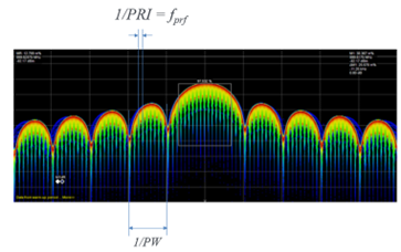 Figure 3
Determining the Target Distance
At this point it is now worth talking about range ambiguity and target resolution. A long duration pulse can propagate over a longer distance, but the trade-off is that you lose the ability to discriminate between two targets that are close together. A short duration pulse will not propagate as far but you gain the ability to discriminate between two targets that are close together.
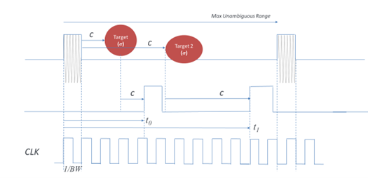 Figure 4
Referring to Figure 4 a pulse is aligned to a clock signal. This clock signal defines the resolution of the Radar, and its period is the reciprocal of the bandwidth of the pulse. The clock effectively quantizes the range; each quantized element is referred to as a range bin.
The repetition rate of the pulses (PRI) defines the unambiguous range. This defines the distance the radar can accurately measure, the further away the target, the longer the radiated transmitted pulse takes to return. So, if the return time is longer than the pulse repetition interval (PRI) then the targets distance will be incorrectly measured, its distance is ambiguous. Extending range is achieved by decreasing the PRI. Also, if we have a long pulse and two targets are close together, they may appear in the same range bin.
Referring to the range equation - if the radar needs to detect signals at a distance, then it needs a low bandwidth signal (long duration pulses) and a low frequency. If we also want to have good unambiguous range, then the pulse repetition interval needs to also have a long duration. As range bin time is proportional to the reciprocal of the bandwidth, (again long duration pulses have low bandwidth) then the range resolution of this type of radar, i.e. the ability to measure target distance accurately, and the ability to discriminate between two or more targets close together is poor.
Long range radars with poor range resolution are used for long distance search applications, while they can detect targets at distances of hundreds of miles, they do not have the resolution to be used for accurate tracking and fire control applications.
Better resolution for tracking and fire control is achieved by using shorter pulses (high bandwidth) and shorter pulse repetition intervals, increasing the range bin frequency increases the resolution. The trade-off is this type of radar has long distance target range ambiguity, and its propagation range is significantly reduced as it utilizes higher bandwidth signals, that also require higher carrier frequencies.
To overcome the relationship between pulse width and range resolution modulation techniques can be used. What if we swept the transmitter frequency through the duration of the pulse?
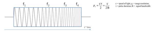 Figure 5
In Figure 5 the RF pulse contains a linear frequency sweep, or LFM (Linear Frequency Modulation), often referred to as a Chirp. This effectively gives us the benefits of a long duration pulse, especially with respect to having the ability to easily amplify, with the resolution a short duration pulse has. At the receiver if we pass this signal though a set of matched filters, we can effectively create the equivalent of a high-resolution short pulse.
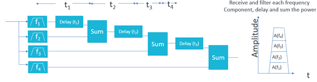 Figure 6
Figure 6 simplifies the matched filter concept discussed above. In figure 5 the signal was split into 4 frequency bands, f1, f2, f3 and f4. In figure 6 we use a bank of filters in the receiver to pass each band and add a delay equal to the duration of each frequency band and sum the amplitudes we end up with an effective ‘stacked’ amplitude pulse of a short duration. This type of technique is used when the highest range resolution is required.
When high resolution is required exclusively, for example active homing techniques used in a surface to air missile engagements or in automotive radar applications an FMCW variant of the above is used, Consider figure 7a. A linear frequency ramp is generated using a VCO (voltage-controlled oscillator). Using a coupler, a fraction of the signal’s amplitude is fed to a mixer as a Local Oscillator (LO), while most of the power is fed through a circulator and transmitted. The reflected much lower power signal is also fed to a mixer and the frequency are subtracted utilizing the non-linear characteristics of the mixer producing an IF (intermittent Frequency) signal.
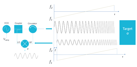 Figure 7a
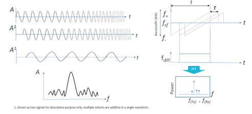 Figure 7b
The as the mixing process effectively subtracts the two signals in the frequency domain, we end up with signal that represents the frequency difference of the transmitted signal and the received signal. (Figure 7b) Preforming an FFT on the signal will produce a frequency component that is proportional to the distance of the target. The wide the frequency sweep, the higher the resolution. A modern automotive system will use a 4GHz sweep, that needs to be transmitted at 77GHz, while this gives excellent resolution if we refer back to the radar equation the range of this type of system is limited to a few hundred meters due to the reciprocal effects of the bandwidth and carrier frequencies.
Figure 8 shows the different types of radar and how the tradeoffs discussed so far are managed, a long-range radar can detect targets at a distance, however the system is very large due to the large antenna required and the resolution is poor due to the smaller bandwidths available at lower frequencies. Tracking and Airborne Radars are higher frequency, and more compact with smaller antennas, have good range resolution and can track targets adequately in the tens of miles range, using a combination of radar mode such as variable PRI’s and utilize both unmodulated pulses and Linear Frequency Modulated Pulses (LFM) depending on the range of the engagement. Radar absorbent designs (Stealth) are usually optimized for these frequency ranges. For very shortrange applications (<300m) a high-resolution wide bandwidth LFM is used. The bandwidth requires a high carrier frequency, (small wavelength), while these systems are very small, can fit in the cone of a missile, or the front of a car the range is restricted to a few hundred meters.
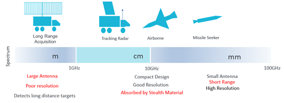 Figure 8
Measuring Target Velocity
So far, we have only discussed the measurement of distance. A radar can also measure the velocity of a target by taking advantage of the Doppler Effect. What this means a frequency difference can be observed between the transmitted signal and the received signal, and it can be measured to determine the velocity of the target and determine if it is approaching the radar or moving away from the radar.
The frequency difference is equal to two time the velocity, dived by the wavelength and compared to the carrier frequency of the radar is a small very small frequency increment or decrement. Again, like target distance the Doppler frequency can also be ambiguous. If the doppler frequency is greater that the pulse repetition frequency (PRF) then the measurement will be incorrect, and the maximum velocity cannot be more than the wavelength multiplied by the PRF.
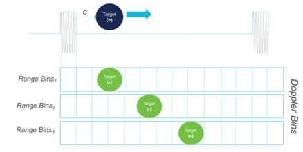 Figure 9
As the doppler frequency is very low compared to the carrier frequency we must measure it over number of pulses. Earlier we discussed the concept of the range bin for measuring distance, to measure Doppler we must observe the small frequency difference over a number of range bins, effectively creating a two-dimensional matrix, the horizontal containing the range bins and the vertical containing the Doppler bins. This is Shown in Figure 9.
Determining the Target Position
We can measure distance and velocity, but how do we know where the target is? One technique is to mechanically move the Radar, so the beam covers a large area. The traditional depiction of a radar is a rotating antenna. The antenna can rotate in a circular fashion, say at about 5 RPM detecting targets in a horizontal plane (Azimuth), or alternatively can move up and down detecting targets in a vertical plane (Elevation). While a mechanical approach can be good for long distance targets when resolution is not an issue, more elaborate techniques need to be employed for higher resolution radars.
For fire control we need to keep the target within a boresight. One method is to mechanical rotate the bean conically around the boresight. If the target moves out of the boresight the radar would detect that the target has crossed beam, and mechanically move the fire control system to put the target back in the boresight.
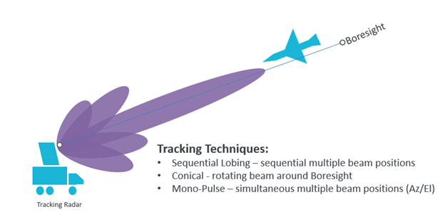 Figure 10 – example of a fire control radar
Mechanical systems and small antenna arrays for search and fire control have been used for many years, however modern radars tend to use more sophisticated ecteronic techniques to determine locations. For fire control a Mono-Pulse system is employed – this utilizes simultaneous multiple beam positions allowing azimuth and elevation to be calculated, however the array needs to be pointing in roughly the correct direction. AESA radars, or Active Electronically Scanned Array is a phased array antenna, which is a computer-controlled array of antenna elements in which a beam of radio waves can be electronically steered to point in different directions without moving the antenna. Wide sweeps of the sky and multiple radar modes and missions can be accomplished by a single AESA radar.
Radar Target Generator
When verifying mission readiness of a new Radar design a Radar Target Generator is often used. An RTG receives the Radar under tests signals, then adds ranges, speed, cross-section, and clutter to this signal and retransmits the signal back to the Radar, thus emulating a real-life target or set of targets performing a complex scenario. This is more cost effective than live range testing.
There are many types of RTG, ranging from a simple delay line, repurposing of an existing Radar or the utilization of a DRFM (Digital Radio Frequency Memory) based system that employs high speed RF DAC’s and ADC’s controlled by an FPGA.
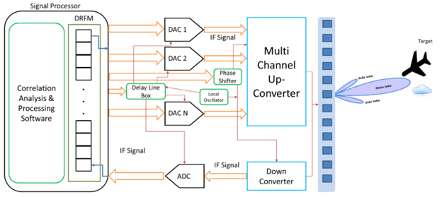 Figure 11 – RTG block diagram
The Tabor Proteus AWT
An Arbitrary Waveform Transceiver is a class of products that takes advantage of the latest RF DAC and ADC technology, combined with high-speed FPGA control and processing to solve complex measurement and simulation problems in Quantum Physics, RF Semiconductor Test, Radar and Electronic Warfare. Its block diagram is like a DRFM system but has a simplified control and setup system allowing targets and scenarios to be setup easily.
The Proteus Family of products from Tabor Electronics, have high performance specifications making it the industry leading Arbitrary Waveform Transceiver. It is a modular based solution based on the PXIe standard and comes in three form factors to suite your applications need - Module, Bench and Desktop.
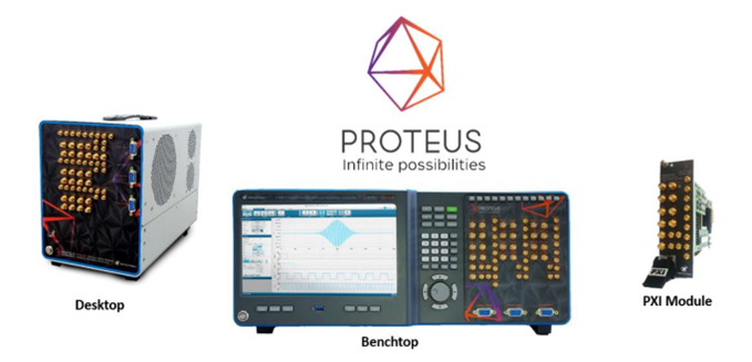
The Tabor Proteus AWT (Arbitrary Waveform Transceiver) series comes with a unique architecture of combination of AWG & Digitizer on a single FPGA, as shown in Figure 12
Its modularity allows for configurations of multiple channels RF beams, either emulating Mono-Pulse or AESA Radar, or creating multiple target scenarios.
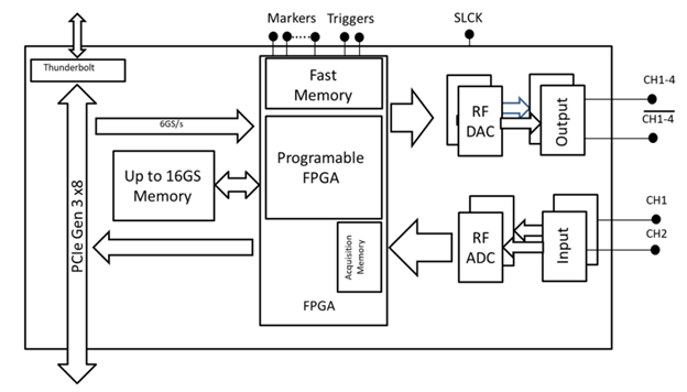
Figure 12 – The Tabor Proteus AWT
Proteus Key Features
- Up to 4 channels and up to 9 GSa/s DAC sample rate
- Up to 16 bits DAC resolutions
- DUC/NCO mode for RF up conversion on all channels
- Skew between channels < 25ps
- Up to 2 digitizer channels per module
- Up to 5.4 GSa/s sample rate
- 12 bits ADC vertical resolution
- DDC mode for RF down-conversion on all channels
- Loopback mode
- Loop delay down to 400ns
- Direct streaming to DAC
Tabor Proteus AWT as an RTG
Proteus series RF Arbitrary Waveform Transceivers have a very compact size and form factor. Each base module has 4 phase synchronous DAC channels enabled with DUC and 2 phase synchronous ADC channels equipped with DDC features.
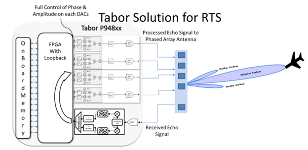
The ADC channels will receive the echo pulse reflected from the target and will pass through the DDC as shown in the above setup. Operation in multiple Nyquist Zone can be achieved from low frequency to X-Band. For higher fidelity and eider frequency performance the Proteus AWT can be used with external IQ modulators/demodulators and the LUCID series of Local Oscillators.
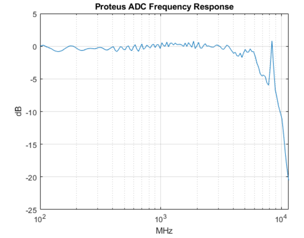
Wide Bandwidth Operation
The tabor AWT supports signal creation of up to 2GHz BW using the DAC and 2.7GHz with the ADC. Fast phase coherent frequency hopping can also be implemented within the bandwidth of the DAC and ADC.
Summary
The Proteus series of AWTs have been designed to operate as both radar signal generation/simulation devices and with the optional digitizer as an analysis tool as well. Utilizing the FPGA full real-time loop back is also possible.
- Standalone radar signal generator.
- In loopback – Arbitrary Waveform Transceiver mode.
- Streaming data directly to a DAC.
- FPGA shell mode which gives the user flexibility to configure the operation of the internal FPGA.