Introduction
Creating and analyzing signals with Proteus and MATLAB takes a few simple steps. In this application note we show how to generate and receive a WLAN beacon signal at 2.4GHz in the instruments' first Nyquist Zone. The code can easily be modified to create a signal in the second Nyquist zone, all the way up to the WiFi-6 frequency extension of 7.125GHz.
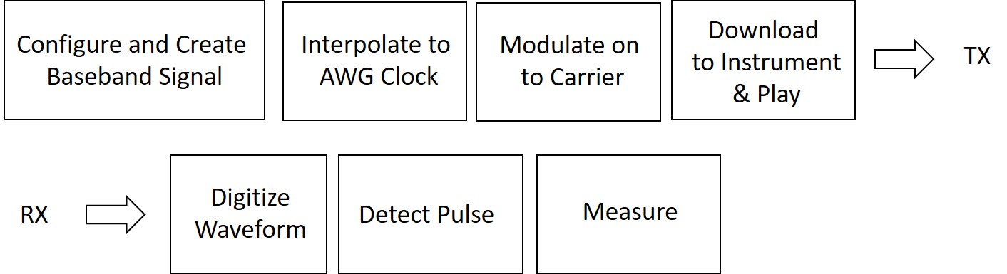
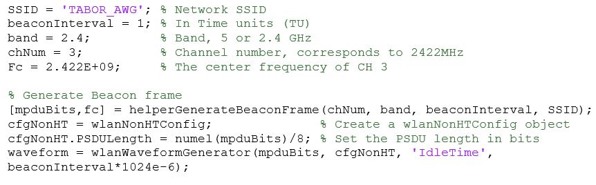
Configure and Create the Baseband Signal
The beacon frame is a type of management frame. It identifies a basic service set (BSS) formed by a number of 802.11 devices. The access point periodically transmits the beacon frame to establish and maintain the network. The beacon frame consists of a MAC header, a beacon frame body and a valid frame check sequence (FCS). The beacon frame body contains the information fields which allows stations to associate with the network. A WLAN beacon frame is created using the wlanMACFrame function. We use the helper function helperGenerateBeaconFrame and we configure for non-high throughput operation. The beacon frame is encoded and modulated using the wlanWaveformGenerator function to create a baseband beacon packet.
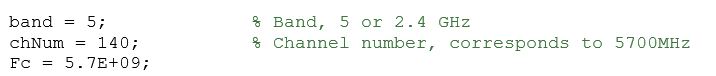
5G Band operation
Plotting waveform yields the following result:
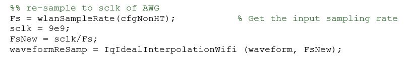
Interpolate 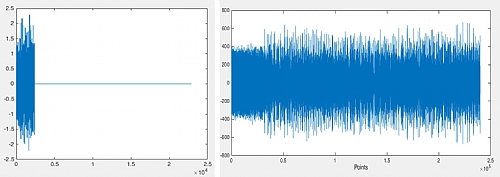 to AWG Clock
The sample rate is 20MS/s, and this directly equates to 20MHz of signal Bandwidth. For first Nyquist operation we can set the instrument's sample rate to 9GS/s. In the example we define Fs as the sample rate of the baseband signal and sclk as the sample rate of the instruments sample clock.
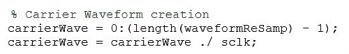
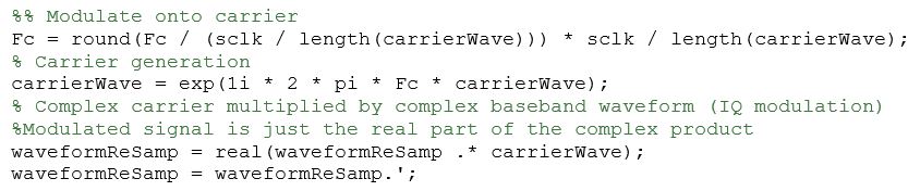
Modulate onto carrier
First, we create the carrier wave array;
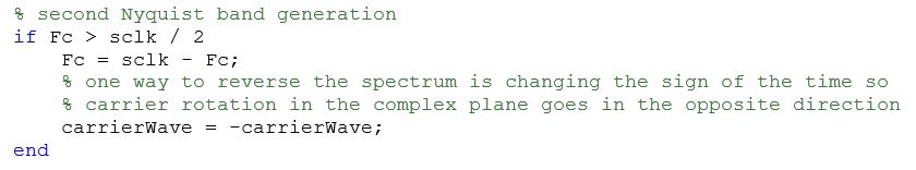
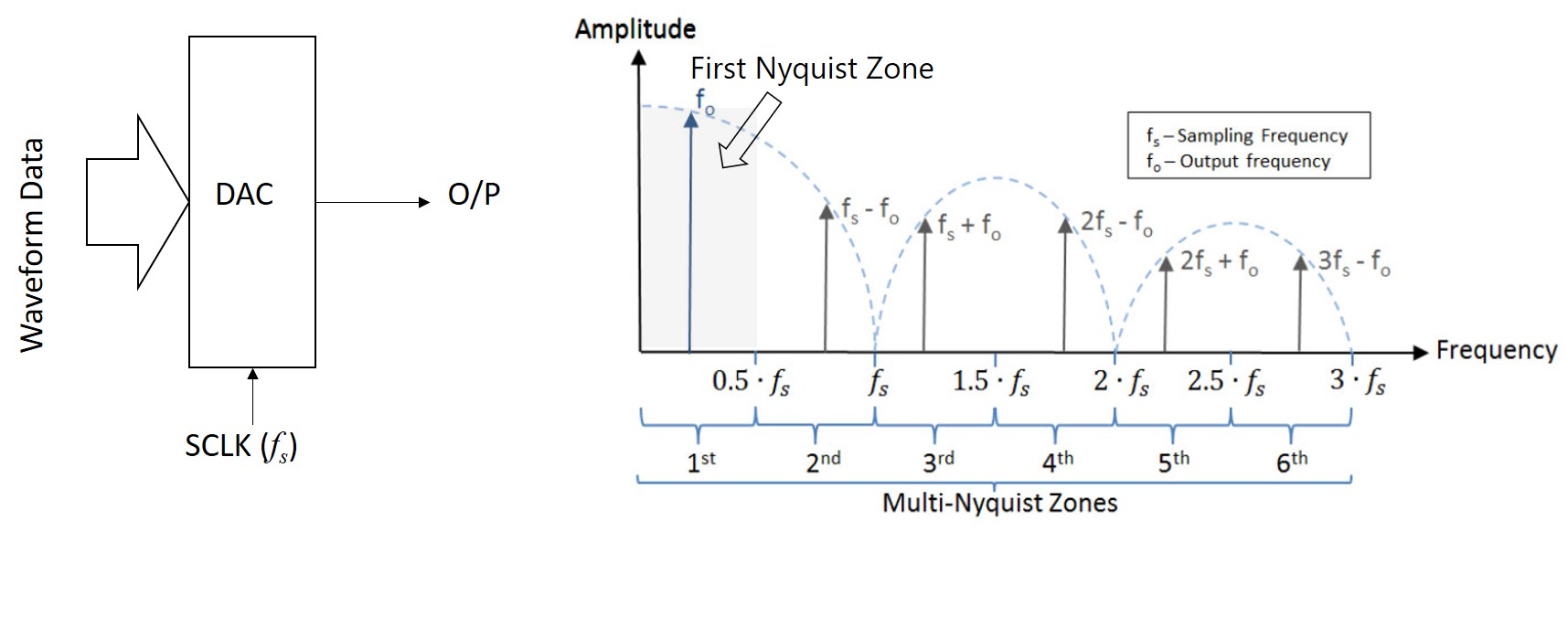
If we want to generate a signal in the 5G-band we will generate the signal in the second Nyquist zone. Referring to the figure bellow - Fc would calculate as follows Fc = sclk - Fc; or 3.3GHz in the first Nyquist and 5.7GHz in the second Nyquist. A high pass filter could be used to attenuate the signal at 3.3GHz.
Finally, the following code creates the carrier and modulates the interpolated baseband signal on to the carrier Fc.
Next we format and scale the waveform in preparation for download;

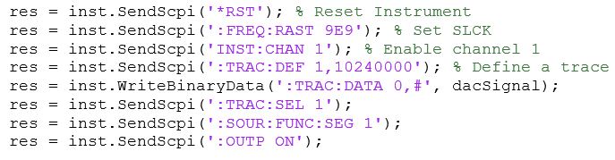
The signal dacSignal is now ready to be downloaded to the instrument.
Digitize the Waveform
We will digitize the waveform using the Nyquist Zone principles discussed earlier. We do this as the maximum sample clock frequency of the Proteus Digitizer is 5.4GS/s. This means the that 2.7GHz is the theoretical frequency limit within the first Nyquist Zone. Our Transmit signal is 2.442GHz, while it falls within the theoretical range, at 2.7GHz you would only get 2 sample points per period. 2.442GHz offers a few more sample points per period more. A more logical approach, and one that would yield in improved signal fidelity, would be to set the sample clock to 2GS/s.
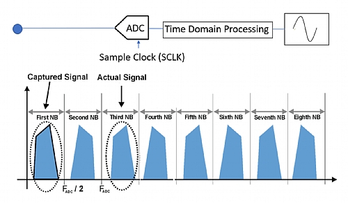
Refering to the above figure – when we sample a 2.4GHz signal with a 2GS/s clock (FADC or SCLK ) we will see an undersampled image of the signal in the first Nyquist Zone or at 400MHz (2.4GHz-2GS/s).
The following code sets the ADC up for an acquisition.
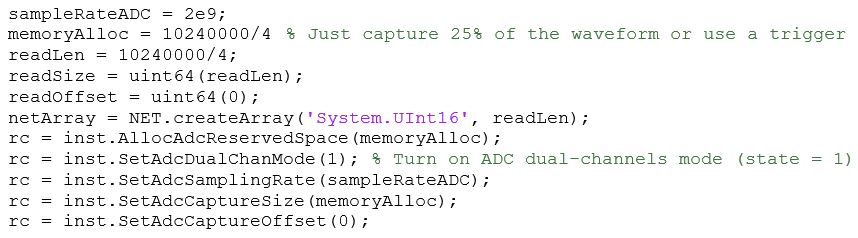
The following code executes the acquisition and stores it in the memory we previously allocated.
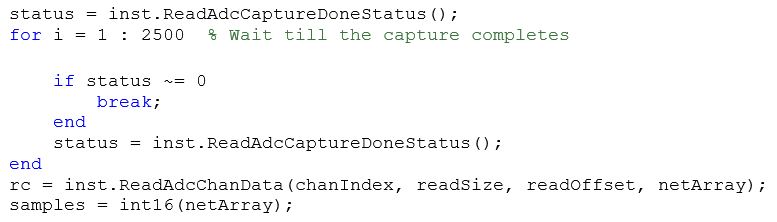
This results in 2.5 million samples being stored in the int16 variable samples. With our sample clock set to 2GS/s this is 1.25ms of captured data.
Detecting the Pulse
In the simple example of acquisition explained above we randomly trigger the acquisition and set a capture time that has a high probability of capturing the pulse. Using one of the many trigger functions of Proteus we could use an external trigger and set a capture time that is equal to the pulse length, or trigger on the pulses own first rising edge and gain set the capture time to equal the pulse length.
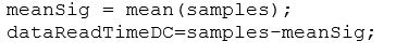
Our capture is stored as a 16bit integer number. The peak values are < 216 and the minimum values are just above zero so one of the first things we should do is normalize samples so the waveform is oscillating around zero. An easy quick way to do this is to take the mean value of samples and subtract it, effectively reducing the inherent DC level and preparing it for the measurement.
Making a Measurement
Now the signal is ready to perform measurements. In the following example I’ve created 4 plots. The first upper left quadrant is the time domain display of the base acquisition, then in the second upper quadrant using a simple software trigger I capture only the pulse itself. The lower plots are broad spectrum 0-1GHz and tuned spectrum with a center frequency of 442MHz.
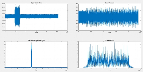
The above plots also have random noise added and I used a filter to eliminate any spurious signals. More measurements are possible using the rich signal processing toolset within MATLAB including modulation quality, adjacent channel power and CCDF.
Conclusion
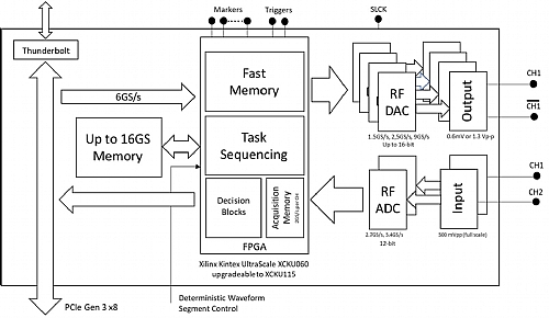
The unique architecture of an AWT allows for wideband signal generation and analysis. The Proteus system uses the latest ADC’s and DAC’s combined with a powerful FPGA that we can also utilize for further signal processing.
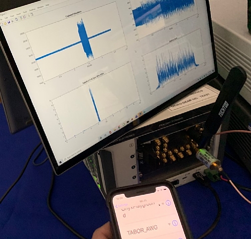
Finally, just for fun we can put an antenna on the differential output of the AWT and see if we can pick-up the beacon signal!
The code examples can be found on our Github site – please provide us with your Github name and we will authorize you as a collaborator.
For more information info@taborelec.com