3 Advantages of DUC for RF signal Generation in AWGs
Waveform Memory Size and Overall Waveform Data Transfer Rate
The gains in terms of waveform memory efficiency when DUC is used to generate RF signals (thanks to the usage of interpolation) has already been mentioned. However, these gains go beyond what can be expected from the mere reduction of the incoming sample rate for baseband waveforms. Generating accurate RF signals through direct generation of the carrier is not as straight forward as it could seem. For a continuous modulation, the waveform must be calculated in such a way it can be looped seamlessly. This requires an integer number of symbols, an integer number of carrier cycles, and an integer number of samples. Some modulation schemes may require the number of symbols in the sequence, to be a precise number in order to be meaningful for the receiver under test. Additionally, the waveform length must be always a multiple of a given number in high-speed arbs as samples are read in parallel from the DDR massive memory. The above considerations may result in the need to round the actual symbol rate or carrier frequency to the closest value resulting in the required waveform continuity conditions. An example can help to understand this issue. Let’s take a DVB-T signal (8MHz channel BW, symbol duration 924ms for 1/32 guard interval) for basic receiver test at UHF channel #69 (858MHz). A minimum consistent DVB-T signal, so the receiver can recognize the modulation parameters, requires a complete sequence of TPS carriers (these carriers supply the modulation parameters for the DVB-T signal), made of 32 OFDM symbols. Let’s generate such a signal through direct generation of the modulated RF signal, at 9GS/s with an AWG with a 64 samples waveform length granularity. The first thing to do is calculate the duration of the 32-symbol sequence:
Time Window (TW) = 32 * 924ms = 29.568ms
The corresponding waveform length can be calculated:
Waveform Length (WL) = SR * TW = 266,112,000 samples
Fortunately, this number is already an integer and a multiple of 64 so the length does not have to be rounded to the nearest integer multiple of 64 (that should change the accuracy of the symbol rate up to 0.12 ppm), or repeated in memory until an integer multiple of 64 would be obtained (no symbol rate error in this case, worst case would lead to repeating the same sequence of samples up to 64 times, so more than 17G Samples would be required).
Next step is calculating the right carrier frequency so an integer number of cycles for the carrier will be obtained:
Number of Carrier Cycles = TW * CF = 25,369,344
Again, the number of cycles at the target carrier frequency is an integer so the carrier frequency will be accurately generated. If this is not the case, adjusting the number of cycles to the nearest integer could result in a 17Hz error for the frequency carrier.
Let’s take now the case of the same AWG using a DUC with 8X interpolation. This interpolation results in a baseband sample rate of 1.125GHz so modulation BW is around 1GHz, more than enough for this DVB-T signal. Calculations must be repeated for the new conditions:
Waveform Length (WL) = 33,264,000 samples
This is an integer number multiple of 32 (granularity is halved for complex signals stored as interleaved IQ pairs) so there is no need to round the number or repeat the sequence within the waveform memory. As the NCO frequency is what determines the carrier frequency, the only important consideration is the frequency resolution of the NCO, which is typically in the tens of mHz range. The gain in terms of waveform memory usage is a factor of four (complex samples are made of two real samples each). Even more, any FC error coming from a frequency error in the sampling clock can be corrected by setting up a corrected FC in the NCO. The only way to do so is by modifying the sampling rate itself.
Carrier Coherence
The above considerations are also important for pulsed signals (i.e. radar) if carrier coherence must be maintained between RF bursts (fig. 3.1). Keeping carrier coherence is important in multiple applications. Coherence requires preserving frequency and phase during all the testing time. Using direct generation of the RF carrier (no DUC), may be difficult, if not impossible, depending on the signals being generated. In a WiFi sequence of packets being made of waveforms segments of different lengths, the number of cycles of the RF carrier for all the RF bursts might not be an integer number for all of them. As these signals are bursts, it looks like keeping the number of cycles being an integer number may not be necessary. However, a careful analysis shows that the phase of the carrier will change from segment to segment, which is not acceptable for some applications. The NCOs in the DUC keep going independently of the waveforms being sequenced, so the right coherent phase is maintained, as long as the NCO is not reset. Another situation, where direct carrier generation may result in the loss of carrier coherence, is when segment generation is asynchronously started through software, or hardware trigger events. Again, the NCO independence of the waveform memory reading process, makes coherence possible no matter the way waveform segments are triggered or sequenced.

Figure 3.1: Many applications require keeping the coherence of the carrier indefinitely. Direct generation of the carrier embedded in the waveform does not guarantee coherence unless the carrier frequency is limited to one resulting in an integer number of cycles within a segment. Even in this case, coherence is only kept when segments are seamlessly generated. For asynchronous generation (i.e. after some external trigger event) coherence will be lost as seen at the top. As NCOs in DUCs run independently of the modulating waveforms (doted pulses), coherence is kept no matter what, as seen in the bottom trace.
Quantization Noise Dithering
When AWGs generate continuous RF (or non-RF) waveforms by looping the same segment over and over again, an interesting effect occurs (fig. 3.2). Quantization noise, generated even by perfect DACs and seen as a random process when dealing with real-world signals, becomes periodic. Quantization noise can be modeled as a constant distribution white noise with one LSB peak-to-peak amplitude. Ideally, the SQNR (Signal-to-Quantization-Noise Ratio) for a sinewave using the full DAC range depends on the resolution in bits of the DAC:
SQNR(dB) = 6.02 x N + 1.76, N = DAC resolution in bits

Figure 3.2: When looping a waveform, such as a multi-tone signal, quantization becomes periodical, and it shows as a series of discrete tones (a). If the waveform length holds multiple cycles of the waveform without repeating the same sample sequence, the repetition period grows, and the average power of the tones is reduced at the price of a longer waveform (b). As carriers generated by the DUC do not have to be synchronous with the waveform, the repetition period of the waveform can be extended to hours, days or weeks. As a result, quantization noise becomes denser and the best possible SFDR is accomplished (c).
The fact that quantization noise becomes periodic, has a major impact on the spectrum of that noise. While quantization noise in operating devices (such as a CD player or a Wi-Fi transmitter) can be modeled as random, so its spectrum is dense and evenly distributed, quantization noise for repeating waveforms shows up as discrete spectral lines located at multiples of the repeating frequency). The average power level of these discrete tones depends on their number, as total power remains constant, as depicted in the expression above. In other words, the shorter the signal, the bigger the distance between those quantization noise tones, and the higher the average power of them. Eventually, these tones can show up over the background noise and be a major contributor to the reduction of the SFDR performance, modulation quality degradation, and ACPR. Just to show an example of this, let’s consider a satellite link QPSK signal at 25.776MBaud (51.552Mbps) generating a PRBS7 test sequence. As a PRBS7 sequence is made of 27-1 = 127 bits, the same sequence of bits must be repeated twice to fit an integer number of QPSK symbols (2 bits /s symbol). The minimum sequence of symbols will be then 127. This means that the minimum TW for this signal will be:
TW = 127 / 25.776 x 106 = 4.927ms
This will result in a repetition rate of 203KHz and, therefore, quantization noise will show up as harmonics of that frequency. One way to reduce the average power of these tones is by increasing the sampling rate when possible, as the noise will be spread over a higher BW. When this is not feasible, it is possible to reduce the average power by reducing the repetition rate. This cannot be done by simply appending multiple copies of exactly the same waveform in the memory, because this will not change periodicity. There are two ways to handle this situation when direct RF carrier generation is involved:
- Calculating a new waveform where the multiple repetitions of the same basic waveform are not sampled in the very same sampling instants. A way to make sure this happens would be selecting a waveform length, which does not have any common divide with the number of symbols in a basic sequence. This way, the signal will not repeat exactly in the same way within the waveform, and the noise will be spread over a larger number of tones.
- The second technique is dithering. In this scheme, the same basic sequence of samples is repeated, and then a random number (1/2 quantization level peak-to-peak amplitude is enough) for all the samples. As a consequence, quantization noise will not repeat until the complete segment is looped, and the average level of the quantization tones will be reduced, at the expense of increasing the overall noise in the signal.
Procedure #1 is better as it does not increase the noise power in the system. The best way to proceed is selecting the number of repetitions of the same symbols sequence to be a prime number, and then calculating a suitable sampling rate and waveform length so the latest is not a multiple of the prime number. In this way, no exact repetitions of the same sample sequence will occur in the segment, and the repetition rate for the quantization noise will be reduced by the same prime number factor. If we apply this approach to the AWG used in the previous example and the DVB-S test signal mentioned above, we can calculate the generation parameters for the maximum FDAC = 9GS/s. The TW for one consistent sequence of symbols (127 QPSK symbols) is around 4.927uS. If we use the exact numbers and the target sample rate for 101 repetitions (prime number), the waveform length will be:
WL = 4,478,701 samples
We will use the closest multiple of 64 (the WL granularity for this AWG) lower than the above WL:
WL’ = 4,478,656 samples
Selecting a lower number is convenient as the Sampling rate can be reduced a little bit (from 9GHz down to 8.999909572 GHz) to keep the right baud rate. Reducing the effects of quantization noise in this signal, when using an AWG equipped with a DUC, is much easier as the waveform going to the DAC is not the one in the waveform memory, but the mixing of it with the real-time quadrature sinewaves being generated by the NCO. If the frequency set in the NCO is not an exact integer multiple of the repetition frequency of the sequence in the waveform memory, the sequence will not be the same all the time and, as a consequence, quantization noise will be spread densely over the full spectrum and no noise tones will be visible. Repetition period for the output samples after the DUC block can range
from seconds until weeks, so at the operational level, it will behave as an ideal white noise without increasing the overall noise level. In this case, it means that the WL could be kept to the minimum 44,288 samples.
Processing Gain, Effective Bits, and DAC Modes
Probably, the most important bottleneck for high-speed arbs is the DRAM to DAC interfacing. Even when using massive parallelization, the sustained transfer rate to the DAC is limited. This results sometimes in a trade-off between DAC resolution and sample rate as the product is the sustained data rate between memory and DAC. For a 9GS/s, 8-bit resolution DAC, transfer rate is 9GByte/s. For a 2.5GS/s, 16-bit DAC, the data rate will be 5GByte/s. And sometimes this is not the full picture, as some other information may be transferred concurrently from the waveform memory such as markers, so some instruments may lose resolution when markers are activated, as the transfer rate has reached the maximum allowed by the implemented architecture.
DUCs also have an impact on this issue as they incorporate interpolators. When DUCs are implemented right in the DAC block, waveform data being transferred to the DAC block is reduced by half of the interpolation factor (for IQ modulation). If the waveform data transfer rate for a 9GS/s DAC is limited to 5GByte/s it is possible to transfer up to 1.25GSample/s 16-bit IQ sample pairs (so Modulation BW goes beyond 1GHz). The DUC using an 8x interpolation factor can handle such rates when the sample rate is 9GS/s, while direct generation of the RF carrier would be limited to 8-bit samples over 2.5GS/s. Interpolation opens the door to use higher than necessary sampling rates and this results in what is called “processing gain”. Basically, oversampling a waveform by a factor of 4, is like using a DAC with one additional bit of resolution at the original sampling rate (fig. 3.3).

Figure 3.3: Near-Ideal Interpolation (Oversampling) is part of digital up-conversion. Oversampling results in a reduction of the quantization noise power spectral density as the same. Increasing sample rate by a factor of two results in a 3dB reduction in the noise power over the signal’s BW, so it is like increasing the effective number of bits (ENoB) by 0.5.
Simultaneous RF and non-RF signals synchronous generation (Envelope Tracking)
AWGs are general purpose signal generation devices. The DUC mode can be used to generate RF signals conveniently, but the same device must be capable of generating signals through direct conversion, so non-RF signals with DC components can be generated as well. Some applications may require the synchronous generation of both kinds of signals (i.e. envelope tracking or Qubit Control, fig. 3.4). In some AWGs, though, the DUC mode can be activated or deactivated for all the channels simultaneously. Fortunately, it is possible to generate baseband (non-RF) signals through the DUC as well. The procedure is quite simple as it requires setting both the frequency and the initial phase for the NCO to zero, and then use the I samples (Q samples can be set to “all zeros” to reduce digital noise) as the non-RF signal to be generated. As the waveform will go through the same processing blocks in the DUC (oversampling, low-pass filtering, etc.) the synchronization and sampling rate for all the signals, RF and non-RF, will be consistent.

Figure 3.4: AWGs are a very versatile tool as they can generate any kind of signal. In particular, they can generate RF and baseband signals simultaneously. The Tabor P9484M is a good example. Here two channels generate two different AC-Coupled RF signals, and the other two channels generate the corresponding synchronous DC-Coupled “envelope tracking” signals to properly handle a high-efficiency RF Power Amplifier.
Waveform normalization and quantization for DUCs
Baseband IQ signals must be calculated, processed, and transferred in order to generate valid RF signals using a DUC. Especial care must be taken when building those waveforms. First, although the I and Q waveforms can be handled as a pair of waveforms, it is important to keep in mind that those are, in fact, just a single waveform made of complex numbers, and it must be handled in that way. One important issue in AWGs is obtaining the maximum SNR without distorting the signal. This is even more important for RF signals. The usual practice is using the full DAC range, so waveforms are normalized to that range and then the required amplitude and DC level is set using the output voltage and offset controls (fig. 3.5). This is also true when using the DUC. However, the full range of the DAC is now connected to magnitude of the complex signal and not to the amplitude of each of the real and imaginary (or I and Q) components. Normalization to the DAC range must be carried out over the peak magnitude of the complex signal so both signals must be normalized together.
Another issue is the DAC range itself. The DUC interprets the midrange level as 0.0 so the available DAC range goes from 1 (instead of 0) up to 2N – 1. Using the “all zeros” level as the extreme value would result in a small DC offset in both the I and Q components (fig. 3.6). This DC offset will show up as a small residual carrier impairment (visible in a Spectrum Analyzer even for a 16-bit sample). It will also result in a residual RF carrier generated between RF pulses or bursts. Keep in mind that one of the advantages of the DUC architecture is that residual carrier can be avoided and that the “OFF” state for pulsed RF is perfect.

Figure 3.5: When using DUCs in AWGs, I and Q samples are stored in the waveform memory. I and Q samples are combined through the IQ modulator. It is important to avoid DAC clipping as this results in heavy non-linear distortion, spectral growth, and poor modulation quality. In order to avoid clipping, the I and Q waveforms must be normalized in a way that the maximum peak is always below the DAC range.

Figure 3.6: The best way to leverage the full dynamic range of a DAC is by normalizing the range of the waveform so it covers all the quantization levels of the DAC (a). This approach is not perfect when waveform data is normalized for DUC use. It is important to keep perfect symmetry around the “zero level (2N-1 level) so the “all zeros” level (the minimum) must be avoided in order to remove an unwanted residual carrier (b).
Generating Multiple Modulated Carries Through a DUC
Most times DUC are used to generate a single modulated carrier and the carrier frequency is set only by the NCO settings. As previously mentioned, traditional analog IQ modulators are difficult to align, and they generate multiple impairments. Many of these impairments generate noise (or self-interference) within the BW Occupied by the signal. Quadrature errors result in unwanted images (frequency components in one of the sidebands generate interfering signals in the opposite sideband) and components such as carrier feed-through (therefore some OFDM-based standards do not use the central carriers). One way to minimize the effects of those impairments is by shifting the complex baseband signals (fig. 3.7) by rotating them so the final I’ and Q’ waveforms are calculated as follows:
I’ = I x cos (2p FS t) - Q x sin (2p FS t)
Q’ = I x sin (2p FS t) + Q x cos (2p FS t)
FS can be positive (so the Fc > FNCO) or negative (so the Fc < FNCO). If the different FS are properly selected, signals will fit in the available modu higher than half of the modulated waveform BW, no image will overlap and the carrier feed-through will be out of the useful signal. This methodology can be used to combine multiple IQ modulated baseband waveforms so the DUC can generate multiple, independent modulated signals over the available Modulation BW. There is no need to use these tricks to avoid such impairments in DUCs as all the modulation process is numerical, and impairments such as quadrature error and imbalance, and carrier feed-through are, by definition, non-existing. However, when an external IQ modulator is necessary (i.e. to reach higher carrier frequencies), the rotating I and Q components can be generated using a two-channel AWG equipped with built-in DUCs. To do so, just set the two channels to work in the regular DUC mode and set the I component for channel 1 with the I component of the complex signal and the Q component to “all zeros”. Then set the Q component of the complex signal of channel 2 with the Q component of the complex signal and the I component to “all zeros”. Next set the same frequency and phase for each NCO. Frequency must be set to the desired positive frequency shift. For negative shifts, just swap the target for the I and Q components (or the target component for each channel). This arrangement only works if all the NCOs are phase coherent.
The same approach can be used by numerical IQ modulators (or DUC) so IQ signals may be shifted in frequency by rotating the waveform data being downloaded to the waveform memory. As there is no need to do so to avoid IQ modulation impairments in DUCs, the only reason to do so is generating multiple RF signals at the same time within the modulation BW of the DUC (i.e. multi-tone signals). Keep in mind, though, in this case the available DAC range must be shared by all the RF signals, so average power will be reduced as the number of signals grow.
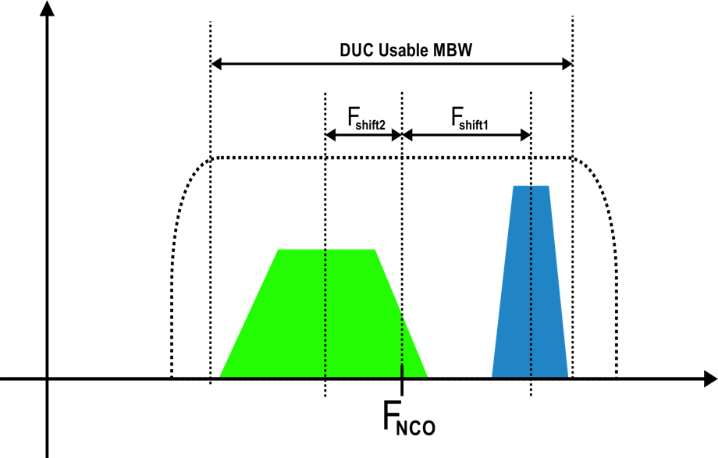
Figure 3.7: Multiple independent, modulated signals can be generated using a single DUC if the full bandwidth of the combined signals fits in the available Modulation Bandwidth (MBW) of the IQ modulator.
To read the next part of the white paper>>
For more information contact [email protected]