Correcting Non-Linear Behavior
SFDR is probably the most limiting factor when using a multi-tone signal for a given test. In previous sections, the best practices to maximize this parameter have been shown and discussed. However, IMD caused by non-linearities will always show up in the final signal. It will be visible as unwanted tones in the adjacent channels or within the notch implemented for in-band testing. In the previous section, the way to characterize and correct linear distortions have been discussed. The key is that AWGs can produce pre-distorted signals that after going through the conversion chain result in undistorted versions of them. Can this concept be applied to non-linear behavior? The answer is yes, with some limits. Theoretically, if the non-linear distortion mechanism was fully known and invariant, the signal stored in the waveform memory could be non-linearly pre-distorted and generated as an undistorted signal at the output. In this case, the problem is knowing the non-linear distortion mechanism, as different sources can show up as similar effects in the output signal. A good example is static non-linearity and dynamic non-linearity. While static non-linearity is relatively simple to determine, dynamic non-linearity may be extremely difficult to characterized and described mathematically and it is not possible to pre-distort a given waveform without this detailed mathematical description.
Multi-tone signals are not any kind of signal and, fortunately, there is some characterization and correction strategy that does not require any knowledge about the distortion generation mechanism. This methodology is known as the Nulling-Tones technique.

Figure 0.1 The nulling tones method consists in characterizing the amplitude and phase of unwanted IMD tones and apply an interfering tone with the same amplitude and opposite phase (as seen in step 3). While measuring the amplitude accurately over a large dynamic range is quite simple, using a Spectrum Analyzer, phase cannot be established directly. Instead, two interfering tones of the same amplitude and two known phases can be applied, and the resulting amplitude measured (Step 1). From the relative amplitudes of both measurements, the unwanted tone phase can be obtained (step 2). This process must be made on all the unwanted tones simultaneously and often it is necessary to iterate the process due to the amplitude readings errors (amplitudes are measured close to the SA’s floor noise).
This method will remove unwanted IMD products, leveraging that these products are relatively small compared to the wanted tones. For this reason, the non-linear behavior of the system being corrected will change gently if the changes in the input waveform are small. The algorithm follows these steps:
- Correct linear response including IQ modulator alignment, if necessary.
- Calculate an uncorrected multi-tone signal.
- Download the multi-tone signal and generate it.
- Measure the amplitude of all the IMD products to be removed (adjacent channels, notch) using a Spectrum Analyzer.
- Add sequentially test tones in phase and quadrature of the measured amplitude to all the frequencies to correct and measure the amplitudes.
- From the I and Q amplitude values, the phase of the unwanted tone can be calculated.
- Add a tone with equal amplitude and opposite phase for each unwanted tone as calculated in step 6.
- Go to step 3 until a number of iterations or some power level after corrections are reached.
The nulling tone will keep updating for each iteration until the required level of tone suppression is obtained. This correction cannot be done in one step, for two reasons. One is that the amplitude accuracy of the SA when performing high dynamic range measurements may be limited. The other is that as all the tones to be nulled change, the overall signal will change as well, and even if the change is relatively small, non-linear effects may be altered. The iterative method makes sure that the changes get smaller and smaller for each step and the nulling-tones will converge to a solution.
Using the technique described above one does not have to know anything about the nature of the tone being nulled, so it can also be used to remove any coherent tone from any other source. Just as linear corrections, it can be used for multi-tone signals generated in any Nyquist band. It can also compensate for non-linearities from any external device such as amplifiers, modulators, or mixers. This capability is extremely powerful when the application requires applying high-power signals, as it allows using limited performance RF amplifiers, see below figure.
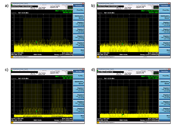
Figure 0.2 The actual output of a 160 MHz BW multi-tone signal at 1.1 GHz directly generated by an AWG can be seen is a). In addition to the wanted tones, there are some IMD products and background noise (most of it quantization noise). In b), the same signal after going through a nulling-tones procedure. The unwanted tones have disappeared under the background noise. In c), the multi-tone signal is generated by using an internal DUC and a complex IQ waveform at a much slower sampling rate. The background quantization noise is greatly reduced. Finally, in d), the same signal is generated using half of the DAC range (6dB attenuation can be observed). Notice that the level of the IMD products is greatly reduced at the expense of a lower amplitude and SNR. Applying the nulling-tones procedure to the signal in c), the same or better level of spurious IMD products could be reached while preserving the precious dynamic range.
Appendix A – Multi-tone Waveform Calculation MATLAB Script
The MATLAB script below calculates a normalized multi-tone signal according to the waveform settings and AWG requirements specified by the variables declared at the beginning. It follows the algorithms described in Error! Reference source not found. Error! Reference source not found., page Error! Bookmark not defined.. The resulting waveform can be exported in a CSV file that can be imported by the WDS or ArbConnection software. It also calculates and displays the PAPR for the calculated waveform along with the spectrum of the signal. Random phase distribution is different each time the script is executed so different values for PAPR can be expected.
%*************************************************************************
%*
%* Multitone Waveform Calculation
%*
%* Author: Joan Mercadé, Application Engineer
%* © 2021 - Tabor Electronics, Ltd
%*
%*************************************************************************
% AWG Settings
samplingRate = 9.0E+09; % Sampling rate for the target AWG
granularity = 32; % Waveform Length Granularity
lengthMethod = 1; % Length calculation method. 1 = round, 2 = lcm
% Multi-tone Settings
numberOfTones = 21; % Total number of tones to be generated
startFreq = 0.8E+09; % Target frequency for first tone (Hz)
toneSpacing = 40.0E+06; % Tone spacing (Hz)
numOfReps = 53; % A HIGH PRIME NUMBER like 53.
phaseDistType = 2; % =0 CONSTANT PHASE, =1 RANDOM PHASE,
% =2 PARABOLIC(NEWMAN), =3 RUDIN-SHAPIRO
% Notch Definition
notchStarTone = 0; % Start tone for notch (1...numberOfTones);
notchNumOfTones = 0; % Number of tones included in the notch;
% Export CSV File Creation
saveFile = false; % Save file
fName = "RefToneFile.csv"; % File name
% Record Length And Parameter Calculation
% Base Freq Resolution
repOfReps = 1;
freqRes = toneSpacing / numOfReps;
% Integer waveform length closest to the required resolution
wfmLength = round(samplingRate / freqRes);
% final wfmLength calculation to meet the granularity requirement
if lengthMethod == 2
repOfReps = lcm(wfmLength, granularity) / wfmLength;
wfmLength = lcm(wfmLength, granularity);
else
wfmLength = granularity * round (wfmLength / granularity);
end
% Actual freq resolution depends on the final waveform length
freqRes = samplingRate / wfmLength;
% Actual toneSpacing depends on the final freqRes
toneSpacing = freqRes * numOfReps * repOfReps;
% Start and final frequencies are calculated
startFreq = round(startFreq / freqRes) * freqRes;
finalFreq = startFreq + (numberOfTones - 1) * toneSpacing;
% Waveform Creation
% Time values are calculated for each sample
xValues = 0 : (wfmLength - 1);
xValues = xValues / samplingRate;
% Amplitude is flat by default (all ones)
amplTable = ones(1, numberOfTones);
% Actual tone frequencies are calculated for each tone
freqTable = startFreq : toneSpacing : finalFreq;
% Phase initialized to tones
phaseTable = zeros(1, numberOfTones);
% Notch Insertion
if notchStarTone > 0 && notchNumOfTones > 0
amplTable(notchStarTone : notchStarTone + notchNumOfTones - 1) = 0.0;
end
% Phase Set Up
% Random Phase
if phaseDistType == 1
phaseTable = 2.0 * pi .* (rand(1, numberOfTones) - 0.5);
end
% Parabolic Phase (NEWMAN)
if phaseDistType == 2
phaseTable = 1:numberOfTones;
phaseTable = 1.0 - phaseTable .* phaseTable;
phaseTable = -(pi / numberOfTones) .* phaseTable;
phaseTable = wrapToPi(phaseTable);
end
% Rudin Sequence (near optimal for 2^N tones)
if phaseDistType == 3
numOfSteps = int16(round(log(numberOfTones) / log(2)));
if 2^numOfSteps < numberOfTones
numOfSteps = numOfSteps + 1;
end
numOfSteps = numOfSteps - 1;
temPhase(1:2) = 1;
for n = 1:numOfSteps
m = int16(length(temPhase) / 2);
temPhase = [temPhase, temPhase(1 : m), -temPhase(m + 1 : 2 * m)];
end
phaseTable = -0.5 * pi .* (temPhase(1 : numberOfTones) - 1);
end
% Multi-tone Waveform Calculation (I/Q)
multiToneWfm = zeros(1, wfmLength);
freqTable = 2.0 * pi * freqTable;
for i = 1:numberOfTones
multiToneWfm = multiToneWfm + ...
amplTable(i) .* cos(freqTable(i) .* xValues + phaseTable(i));
end
% Normalization to the -1.0/+1.0 Range
maxValue = max(abs(multiToneWfm));
multiToneWfm = multiToneWfm ./ maxValue;
% Calculation of PAPR (Crest Factor)
papr = 1.0 / std(multiToneWfm);
papr = 20.0 * log10 (papr) - 3.0;
% File Creation
if saveFile
csvwrite(fName, multiToneWfm');
end
% Plot Spectrum
pSpec = pspectrum(flattopwin(1, wfmLength) .* multiToneWfm);
pSpec = 10.0 * log10(pSpec);
pSpec = pSpec-max(pSpec);
xFreq = 0:(length(pSpec)-1);
xFreq = xFreq / (2 * length(pSpec));
xFreq = xFreq *samplingRate;
plot(xFreq, pSpec);
axis([-inf +inf -80 20]);
title(strcat('Power Spectrum (dBc), PAPR = ', num2str(papr), 'dB'));
For more information contact [email protected]