How to Properly Manage Tabor’s AWG Arbitrary Memory

In this tutorial, we will give a quick start guide on how you can manage the Tabor AWG’s arbitrary memory using a specific set of Standard Commands for Programmable Instruments (SCPI). These are an ASCII-based set of commands for reading and writing instrument settings.

This tutorial will provide a quick introduction to the Tabor WXxx84C Arbitrary memory set of commands and will demonstrate how programmers could maximize their memory management abilities in a quick & efficient manner. Efficient use of the following commands can save precious time when trying to send large quantities of data to your AWG, whether you need to download a large waveform or a large number of smaller waveforms.

All Tabor AWGs have a similar set of basic commands to use. Although The WX2184C has some features which are unique, It is a good example for learning how to program the basics, as it covers most of the features which also appear in all other Tabor Models.

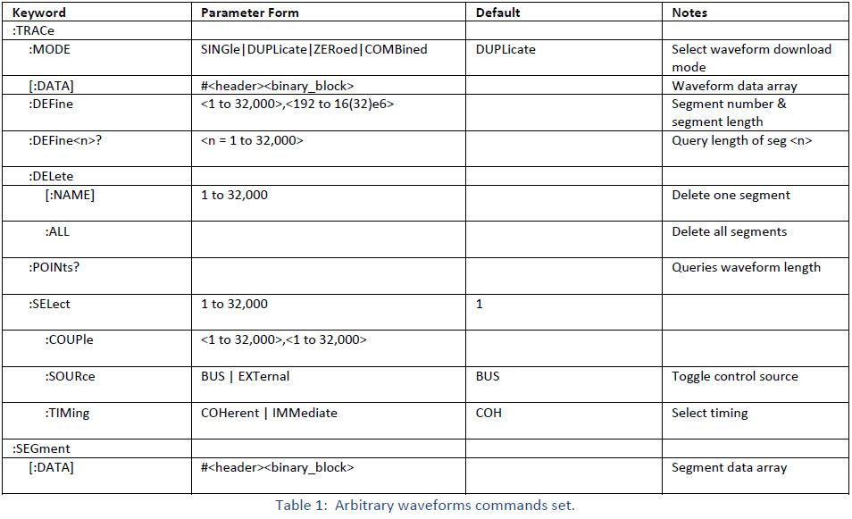
All the arbitrary waveform commands are listed in the Table below. Factory default values after *RST (instrument reset) are shown in the Default column. Parameter range, low & high limits are listed, where applicable. Information regarding each command can also be found in the Tabor user manual, which can be downloaded from Tabor’s website.

 

• Arbitrary Memory Commands - Quick Introduction

Arbitrary waveforms are generated from digital data points, which are read from a dedicated waveform memory and are then converted to analog values using the Digital to Analog Converter (DAC). The values the data points can take depends on the number of bits of the DAC or the “vertical resolution”. In the WX2184C, the vertical resolution is of 14 bits (16,384 points).Hence, each sample is placed on the vertical axis with a resolution of 1/16,384 from 0 to 16383. 

When the instrument is programmed to output arbitrary waveforms, each time the sample clock rising edge occurs, the AWG samples a data point, starting from address 0 to the last address of the segment. The rate at which each point is sampled is defined by the sample clock value. 

Unlike the built-in standard waveforms, arbitrary waveforms must first be loaded into the instrument's memory by the user. Correct memory management is required for best utilization of the arbitrary memory. 

The memory of the Tabor arbitrary waveform generators is comprised of a finite number of points. The maximum memory size depends on the instrument’s model & option. For example, the WX2184C model has 16M/32M memory points for each channel. 

Information on how to partition the memory, define segment length and download waveform data to the Tabor generator using the arbitrary memory commands set is given below. We will go over the technical details of each command one by one, followed by an example of how to properly use this set of commands. It is highly recommended to read the user manual of each specific Tabor AWG model’s you are currently working with.  

1. :TRACe:DEFine<segment_#>,

 

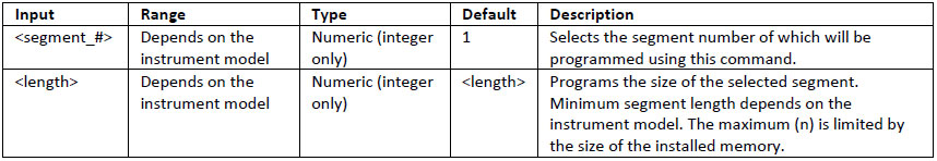
Use this command to define the size of a specific memory segment. In the WX2184C, the final size of the arbitrary memory is 16,000,000 points (32,000,000 points optional). The memory can be partitioned to smaller segments, up to 32Ksegments. The total length of memory segments cannot exceed the size of the waveform memory. Minimum segment size & minimum increment depends on the Tabor model, these restrictions can be found in each of Tabor model’s user manual. For example, for the WX2184C the minimum segment size is 192 with increments of 16 points. 

2. :TRACe:DELete<segment_#> 

This command will delete a predefined segment from the working memory. The memory space that has been released will be available for new waveforms, as long as the new waveform will be equal or smaller in size to the deleted segment. If the deleted segment is the last segment, then the size of another waveform written to the same segment is not limited. 

 

Use this command to set or query the active waveform segment at the output connector. By selecting the active segment, you are performing two functions: 

• Successive TRACE commands will affect the selected segment.
• The SYNC output will be assigned to the selected segment. This behavior is especially important for sequence operation, where multiple segments form a large sequence. In this case, you can synchronize external devices exactly to the segment of interest. 

 

4. :TRACe:MODE SINGle / DUPLicate / ZERoed / COMBined  

 

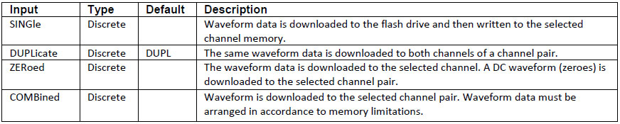
This command will define how the arbitrary waveform is downloaded to the unit’s memory. The output channels of the unit are arranged in pairs, meaning that each two channels share a single memory block of 32Mpoints (64Mpoints optional). The channel pair memory block is divided in such a way that the individual channel’s memory blocks (16Mpoints per channel in standard configuration) are interleaved in blocks of 16 points as depicted  in figure 1 below:

 

As a result of the shared memory block, the segment size of each channel in a channel pair must be identical. In addition, when downloading data, it is ALWAYS written to the shared memory block and therefore to both channels. The user has two ways of downloading the waveform data:

• COMBINED – The Tabor AWG assumes the user is downloading to both channels and has pre-arranged the data in the required 16point interleaved manner. This is the COMBINED download mode and it is the fastest way to download data to the unit. Note that in this mode the user has full control so waveform data must be arranged correctly. 
• SINGLE, DUPLICATE, ZEROED - This second option allows the user to prepare the waveform as if each channel memory is independent and once the data is transferred, the unit itself will arrange the data in the memory. There are 3 modes where the unit handles how the data is written:         

        I. DUPLICATE - When downloading to one of the channel pair, the data is duplicated to the other channel. For example, when downloading a 1024 points Sine waveform to CH1, a 1024 points Sine is also downloaded to CH2.
        II. ZEROED - When downloading to one of the channel pair, the other channel‘s memory is filled with zeroes (DC waveform). For example, when downloading a 1024 points Sine waveform to CH1, a 1024 points DC waveform is downloaded to CH2.
        III. SINGLE - When the data is downloaded to the unit, it is saved to the flash drive and then written to the channel pair memory. This enables the user to download a waveform only to the selected channel without changing data in the selected channel pair.

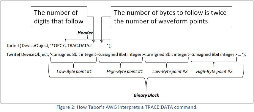
5. :TRACe:DATA#<binary_block>  

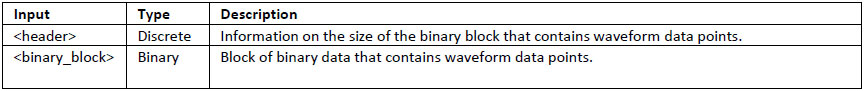
This command will download data to the Tabor’s arbitrary waveform memory. Waveform data is loaded to the WX2184C using high-speed binary transfer, A special command that was defined by IEEE-STD-488.2 for this purpose. This high-speed binary transfer allows any 8-bit bytes (including extended ASCII code) to be transmitted in a message. This command is particularly useful for sending large quantities of data. 

The generator accepts waveform samples as 16-bit integers, which are sent in two-byte words, one after the other. Therefore, the total number of bytes is always twice the number of data points in the waveform. For example, 20,000 bytes are required to download a waveform with 10,000 points. 

Let’s start with a simple example:

fprintf( DeviceObject, ‘*OPC?;:TRAC:DATA#42048’ );

fwrite( DeviceObject, ‘<binary_block>’ ); 

fscanf( DeviceObject,’%d’);

The previous set of commands causes the transfer of 2,048 bytes of data (1,024 waveform points) into the active memory segment. The above command lines are interpreted this way: 

• The ASCII "#" ($23) designates the start of the binary data block. 
• "4" designates the number of digits that follow. 
• "2048" is the even number of bytes to follow. 
• “<binary_block>” represents the waveform data. 
• Proper download of data to the instrument should always start with a ‘*OPC?’ query (operation complete) before the header is sent. The read operation is for the response of the unit once it finishes the download of the binary block.

There are a number of points you should be aware of before you start using the TRAC:DATA command:

I. Each channel has its own waveform memory. Therefore, make sure you select the correct active channel (with the INST:SEL command) before you download data to the generator.

II. Before sending a TRAC:DATA command , you should prepare the Tabor AWG for download by sending these two commands in the following order:

     a) TRAC:DEF command to define a number & length to the segment you are creating (This length should be the same as the number of points you are about to download).

     b) TRAC:SEL command to select the segment number you just created as the active segment. This is done to make sure you are downloading data to the correct segment.

III. When sending the TRAC:DATA command, it is recommended to start the command with a ‘*OPC ?’ query before the header and only then to send the binary data block. In addition, do not use a termination character at the end of the binary block. End the procedure with a read operation for the *OPC? Query.
For example:

For downloading waveform of 1024 points, prepare a 1024 points buffer as follows:

fprintf(DeviceObj, ‘:FUNC:MODE USER;:TRAC:MODE DUPL\n’);
Uint16 data[1024];
for (i=0;i<1024;i++){
data(i) = 16383*(0.5+0.5*sin(2*pi*i/1024)); // waveform data
}
fprintf(DeviceObj, ‘:TRAC:DEF 1, 1024\n’);
fprintf(DeviceObj, ‘:TRAC:SEL 1\n’);
fprintf(DeviceObj, ‘*OPC?;:TRAC:DATA#42048’); // no termination character
fwrite(DeviceObj, data);
fscanf(DeviceObj, ‘%d’);

IV. Each Tabor model has its limitations regarding minimum segment length & minimum increment. For example, using the WX2184C, Waveform length must be a minimum of 192 points with increments of 16 points. Data you will download should comply with these restrictions.

V. It is recommended to first create your waveform data and normalize the values to be in the range of [0, 1]. After you will finish the preparation of your waveform data (creation, adding dummy points), you can maximize the vertical resolution of your waveform according to the Tabor model specifications. For example in the WX2184C, waveform data points contain 14-bit values (2^14=16,384). The range is from 0 to 16383, which corresponds to full-scale amplitude setting. Set the data you wish to download according to the desired resolution.

VI. If you are about to download a large number of waveforms to the Tabor generator, you could save download time by combining all of your waveforms into one data array, download the data using the TRACE:DATA command and then slice it into the proper segments using the SEGM:DATA command. A detailed explanation on how to use the SEGM:DATA command is given in step number 6.

VII. Each data point is a 2 byte word comprised of a low byte and a high byte. The waveform data should be prepared in an array so that for each data point, the generator will accept the low byte of each data point first.

VIII. If COMBINED mode is chosen, the data is written to both channels in each channel pair. It is written in blocks of 16 points alternating between the two channels. Notice that the data must be prepared in the appropriate interleaved manner, 16 points for each channel beginning with CH2.

For example:

For downloading two different waveforms each of 1024 points to a channel pair, prepare a 2048 points buffer as follows:

fprintf(DeviceObj, ‘:FUNC:MODE USER;:TRAC:MODE COMB\n’);
Uint16 data[2048];
for (i=0;i<2048;i++){
if( mod(i,32) <= 15 )
data(i) = 16383; //data for CH2 or CH4
else
data(i) = 0; //data for CH1 or CH3
}
fprintf(DeviceObj, ‘:TRAC:DEF 1, 1024\n’);
fprintf(DeviceObj, ‘:TRAC:SEL 1\n’);
fprintf(DeviceObj, ‘*OPC?;:TRAC:DATA#44096’); // no termination character
fwrite(DeviceObj, data);
fscanf(DeviceObj, ‘%d’);

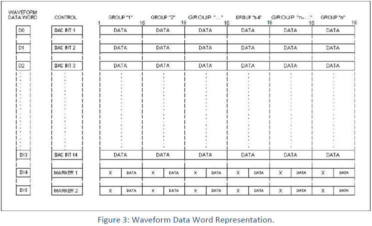
IX. Each data point consists of two bytes, which are 16 bit, but has only a 14 bit value. Markers data is saved in the unused D14 & D15 bits as can be seen in figure 3 below. Marker data is written only to CH2 and CH4. In CH1 and CH3, D14 and D15 are “don’t care”. More information in this manner can be found in the specific Tabor model’s user manual.

6. :SEGMent:DATA# 

The SEGM:DATA command is a very useful SCPI command you would be glad to use in cases you need to partition the waveform memory to a large number of segments. Using SEGM:DATA, one could define an entire segment table in one command, which makes this process extremely fast & efficient. The SEGM:DATA command will partition the waveform memory to smaller segments, hence speeding up the memory segmentation process. The idea is that first, all of your waveform data can be built & downloaded as one long waveform using the TRAC:DATA command and then just use SEGM:DATA to split the memory to the appropriate memory segments. This way, there is no need for definition of waveforms, one by one, to individual segments as with the TRAC:DEF command. 

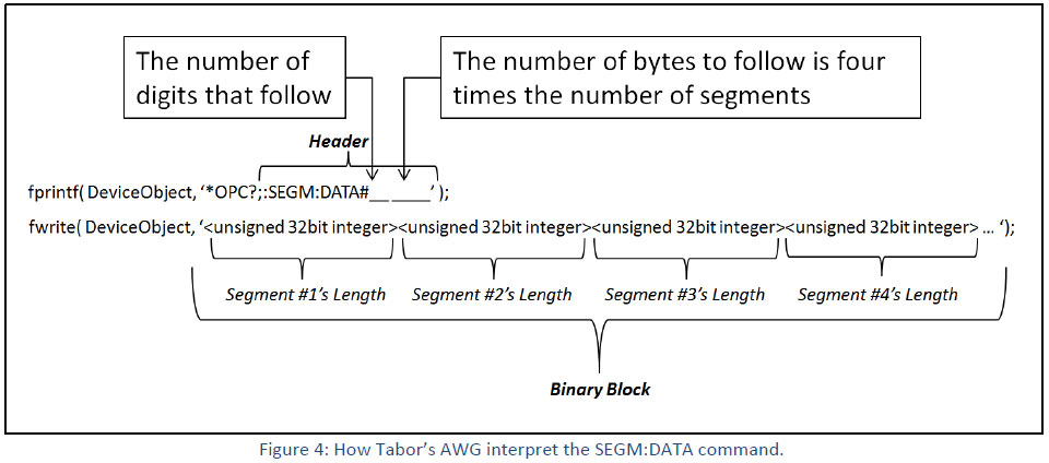
As a simple example, the next commands will download to the generator a segment table of 4 segments: 

fprintf(DeviceObject, ‘*OPC?;:SEGM:DATA#216’ );
fwrite(DeviceObject, ‘’ );
fscanf(DeviceObject, ‘%d’ );

The commands above cause the transfer of 16 bytes of data (4 segments) into the segment table buffer. The command lines are interpreted this way:

• The ASCII "#" ($23) designates the start of the binary data block. 
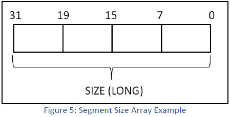
• "2" designates the number of digits that follow. 
• "16" is the number of bytes to follow. Segment table data has 32-bit values of which are used for segment size. Therefore, Data for each segment must have 4 bytes.
• “” contains each and every one of the segment size values in a row. All must be in a 32bit unsigned integer format. 
• Proper download of data to the instrument should always start with an ‘*OPC?’ query (operation complete?) before the header is sent. The read operation is for the response of the unit once it finishes the download of the binary block.

The binary block contains a list of the segments lengths where each segment length is represented using 4 bytes, therefore, the total number of bytes is always 4 times the number of segments. For example, 36 bytes are required to download 9 segments to the segment table. 

There are a number of points you should be aware of before you start preparing the data:

I. Only size is required as input, because segments are automatically numbered. Regardless if you previously had any segments defined, the segment index will start from 1 to n.

II. Each channel pair has its own segment table buffer. Therefore, make sure you selected the correct active channel (with the INST:SEL command) before you download segment table data to the generator.

III. SEGM:DATA command overrides prior segment definitions, similar to the TRAC:DEL:ALL command. Sending TRAC:DEL commands doesn’t really erase the data from the arbitrary memory, it only erases the segment’s definitions (number & length).

IV. Max number of segments depends on your instrument’s model. With the WX2184C, the maximum number of segments is 32,000.

V. When sending this command, it is recommended to start the command with a ‘*OPC?’ query before the header and only then to send the binary data block. In addition, do not use a termination character with this command.

VI. Maximum segment size depends on your installed option. With the basic WX2184C you can program maximum 16M in one segment.

VII. The number of bytes in a complete segment table must divide by 4. The generator has no control over data sent to its segment table during this unique data transfer. Therefore, wrong data and/or incorrect number of bytes will cause erroneous memory partition. In those situations you will be require to reboot.

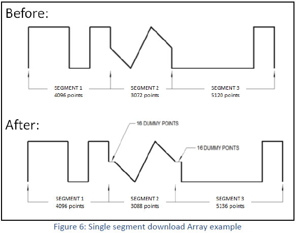
VIII. Due to hardware considerations, when using the :TRACE:DATA command to download several short waveforms as one long waveform, you will need to add 16 dummy points (if minimal segment size is 384, then you will need to add 32 dummy points) at the start of each waveform (except the first) as shown in figure 4 below. Dummy points are points with the same value as the first point of the related segment. This addition must not be added to the total length of the segments. Therefore, this should not be taken into consideration while sending the segments length using the SEGM:DATA.

For example:
Each of the three waveforms shown in figure 6 (besides the first) is artificially expanded by 16 dummy-points right at the beginning of the segment. The value of these points should be the same as the value of the first point of the waveform. So now, the total length of the three waveform segments is 4,000+16+3,000+16+5,000= 12,032 points. To download the data correctly, the download mode should be COMBined.

7. :SEQuence:DATA#

While this command does not belong to this group of commands, it is quite similar to the TRACE:DATA and SEGM:DATA commands. Using the SEQ:DATA one could build a complete sequence table in one binary download. In this way, there is no need to define and download individual sequencer steps using the SEQ:DEF command. Using this command, a sequence table data is loaded to the AWG using high-speed binary transfer in a similar way as when waveform data is loaded with the TRACE:DATA & SEGM:DATA commands. This command is particularly useful for long sequences that use a large number of segments and sequence steps. The number of bytes to be downloaded will be eight times the number of sequence steps: 

 

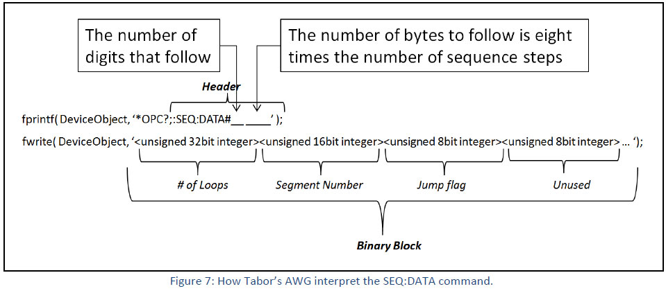
As an example, the next command will generate a three-step sequence with 24 bytes of data that contain segment number, loops and jump flag option.

fprintf(DeviceObject, ‘*OPC?;:SEQ:DATA#224’ );

fwrite(DeviceObject, ‘’ );

fscanf(DeviceObject, ‘%d’ );

This command causes the transfer of 24 bytes of data (3-step sequence) to the sequence table buffer. The binary block contains a list of sequence table entries where each entry is represented by 8 bytes. Therefore, the total number of bytes is always eight times the number of sequence steps. The command line is interpreted this way: 

• The ASCII "#" ($23) designates the start of the binary data block.
• "2" designates the number of digits that follow.
• "24" is the number of bytes to follow. This number must divide by 8.
• “” contains the data of each and every one of the sequence steps in a row:

                     I. Loops as a 32bit unsigned integer.
                    II. Segment number as a 16bit unsigned integer.
                   III. Jump flag as an 8bit unsigned integer.
                   IV. Adding another unused 8bit unsigned integer.

• Proper download of data to the instrument should always start with an ‘*OPC?’ query (operation complete?) before the header is sent. The read operation is for the response of the unit once it finishes the download of the binary block.

8. Coding Examples

Following this tutorial (on Tabor website ->> remote control tutorials) you will find examples attached. The examples are written in MATLAB, Python & LabVIEW and will provide a good introduction to the functionality of Tabor units. Moreover, you will find Python, MATLAB & LabVIEW shared utilities files + interactive examples of how you will be able to use such functions in your own code. Thus, saving you the time it will take to implement them yourself.

In the following example, we created one cycle of sine waveform & divided it into several parts. We then created a sequence, with each of the sine wave parts as a step in the sequence. Each step in the sequence will be generated once to re-create the original sine wave. The example demonstrate how to use faster downloading methods for large number of waveforms & sequences
This example can be found in:

1. MATLAB – “wx2184_Tabor_Example_1.m”
2. LabVIEW – “Using_TRAC_SEGM_SEQ_DATA_SCPI.vi”
3. Python – “wx2184_Tabor_example_1.py”

The example performs the following steps:

I. Creates an arbitrary waveform (1 cycle of a sine wave) with user defined number of points.
II. User will select the wanted segment size and the program will Re-arrange the waveform data by:

• Adding dummy points at the start of each future segment (except the first). 
• Sorting the data string as was mentioned in the TRACE:DATA section of this tutorial ([low byte 0, high byte 0, low byte 1, high byte 1,….]).

III. Partition the waveform memory into the users defined number of segments.
IV. Create a sequence table with each of the segments as a step. Each step will be looped once & the whole sequence will run continuously.

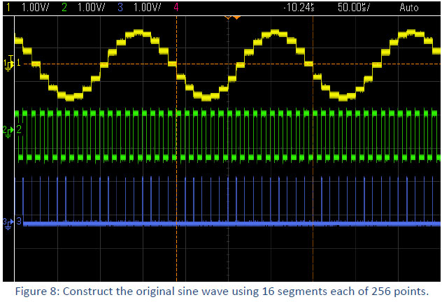
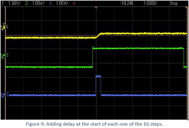
As can be seen on a scope, an example of 4096 sine wave, with additional 16 dummy points was downloaded, the wave was then divided into 16 segments. A sequence table was then created to transmit the segments one after the other each time a valid trigger was applied (we used triggered mode to add a small delay before each step to make the segmentation a bit more visible):

• Yellow - the output sequence.
• Green - the trigger signal.
• Blue – the sync signal

 

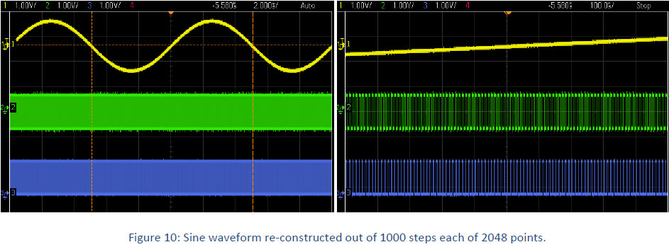
The second time we ran this example we used a 2,048,000 points waveform and divided it into 1000 segments. Here is how it looks on scope:

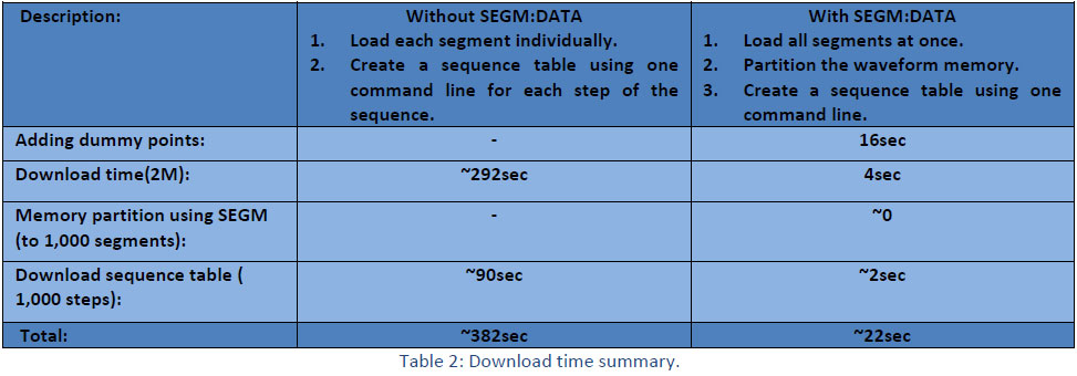
Here is a how much time you could save by using the SEGM:DATA command for managing the Tabor AWG’s memory:

For More Information

To learn more about how to remote control Tabor instruments using Python, MATLAB & LabVIEW, visit our website Support & Tutorials zone. If you encounter difficulties with connecting to Tabor units, please contact us at support@taborelec.com and our support team will gladly help. For more of Tabor’s solutions or to schedule a demo, please contact your local Tabor representative or email your request to info@tabor.co.il.  More information can be found at our website at www.taborelec.com