- Signal Fidelity - Choose the correct sample rate vs waveform characteristics
Any arbitrary waveform generator as the name implies can generate, any type of waveform that you can think of - if it falls within the capability of the instrument. For example, if you wish to generate a 1125MHz sine wave then twice the frequency would seem like an appropriate sample frequency, however at a sample rate of 2.25GS/s there will only be two sample points per-cycle. By increasing the sample rate to 4.5GS/s you get 4 sample points per cycle which is still relatively marginal. Increasing the sample rate to 9GS/s provides 8 sample points per cycle improving the spectral purity of the signal considerably. In all cases a low pass filter can be used to further improve the signal.
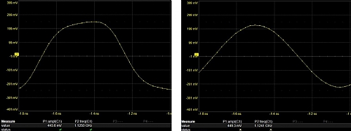
Figure 1: Sample rate set to 2.25GS/s, provides 4 sample points per cycle | Sample rate set to 9GS/s,
provides 8 sample points per cycle
- Improve Fidelity and Frequency Range - Utilize multiple Nyquist Zones
If the maximum sample rate of the signal is 2.25GS/s the spectral purity may be improved by using the instrument in the second Nyquist Zone. If the Sample Rate is set to 1GS/s and a signal of 125MHz is generated – this signal will appear at 125MHz, 875MHz (sample Rate minus 125MHz) and 1125MHz (sample Rate plus 125MHz). In each successive Nyquist Zone, the amplitude decreases, and the spectrum will invert as it goes from one zone to the next.
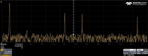
Figure 2: 125MHz Signal in multiple Nyquist Zones (125MHz, 875MHz, 1125MHz, 1875MHz)
- Effective Pulse Shaping by creating signals directly to RF
With high sample rate Digital to Analog Converters as in the examples in sections 1 and 2 above we created signals directly to RF. In some cases, an IQ modulator is available within the instruments digital to analog converter. This allows for easy RF signal generation and modulation as compared to the traditional approach of using a signal generator as an LO and utilizing an IQ modulator. Digital IQ modulation does not require sideband balancing and the nulling of the carrier feed-though, nor does it drift with time.
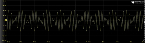
Figure: 3 Using the internal NCO (Numerically controlled Oscillator) to Amplitude Modulate 125Mz waveform file – Time Domain
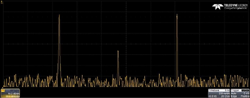
Figure 4: Using the internal NCO (Numerically controlled Oscillator) to Amplitude Modulate 125Mz waveform file
– Frequency Domain
- Understand power, signal to noise and sensitivity.
When you use multiple Nyquist Zones the output power decreases in each successive Nyquist Zone. This usually takes the form of a Sin(x)/x amplitude roll off as show bellow. The signal to noise ratio of the instrument can be approximated to six times the number of bits or more accurately - SNR = (6.02N + 1.76) dB, where N is the number of bits. Therefore with 14 bits of resolution you should get close to 84dB of range and with 16 bits 98dB of range. Other factors will affect range and sensitivity such as spurious and intermodulation. Good frequency planning and filtering can help minimize these.
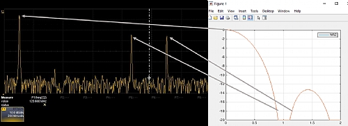
Figure 5: Sin(x)/x amplitude roll off in multiple Nyquist Zones
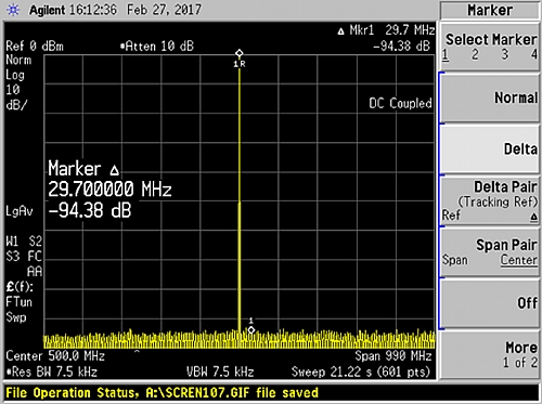
Figure 6: Measured SFDR (Spur Free Dynamic Range) Indicating 16 Bit Resolution
- Multiple channels and multiple instruments – understanding phase
Theoretically if all the outputs of the AWG are derived from the same clock then each output should be phase aligned. Slight differences in each channel analog circuitry may cause a slight timing to offset between channels – this is referred to as the Skew and is often specified in pico-seconds, typically in the order of less than 20ps. The skew can be manually adjusted to an offset of a few nanoseconds with five pico-seconds of resolution. Phase alignment between instruments can is usually more complex and often requires proprietary synchronization and calibration techniques. However, these techniques can yield similar results as with the channel to channel specification, but from instrument to instrument.
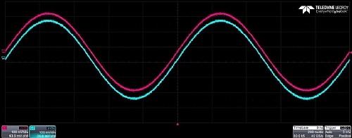
Figure 7: Relative Phase Between two channels
- Determine the correct output stage
Waveform generators often have different output stages. One option is to add a differential amplifier, which will be used to increase the peak to peak voltage range. Another option is to add a Balun to convert the balanced output of the digital to analog converter (DAC) from balanced to single ended. And finally, the outputs of the DAC could be directly connected to the output connectors of the instrument. In some cases, capacitors maybe added for protection, or eliminate any common-mode voltages that the DAC creates. Adding an amplifier will ultimately limit the upper frequency response of the instrument, while adding capacitors will limit the lower frequency response of the Instrument.
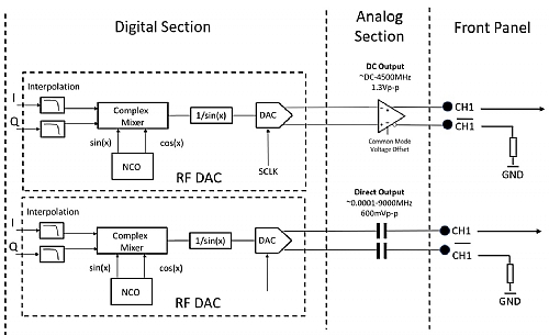
Figure 8: Comparison of DC coupled amplified output vs AC coupled direct output
- Managing Waveform Memory - using onboard memory vs. streaming waveforms in real time
When building complex waveform scenarios, understanding the amount of memory, how the memory is managed and the data transfer mechanism of the waveform to instrument is key. Often instruments with large amounts of Random-Access-Memory RAM (Gigabytes) use Dynamic RAM, this however is much slower than Static RAM by several orders of magnitude. If the instrument has only Static RAM then waveforms can be accessed and played extremely quickly, but memory will be limited to a few 10’s of Mega-bytes. Some instruments employ a hybrid approach utilizing both on-processing-chip fast memory, combined with a large amount of dynamic memory that can be buffered into the fast memory. If the data transfer mechanism is based on a high-speed bus such as PCIe Gen 3, then waveforms can not only be loaded into the instrument very quickly but can also be streamed real-time into the unit. This is useful when there is no a-priori knowledge of the next waveform, for example if it must be calculated based on a previous measurement result.
The following table demonstrates the difference in transfer rates.
| |
x1
|
x4
|
x8
|
|
Gen 1
|
250MB/s
|
1GB/s
|
2GB/s
|
|
Gen 2
|
500MB/s
|
2GB/s
|
4GB/s
|
|
Gen 3
|
984.6MB/s
|
3.94GB/s
|
7.88GB/s
|
Comparison of PCIe generations and lane usage.
Compared to Ethernet 1000Base-T that has a throughout of 125MB/s and USB 3.0 with 4.8GB/s, PXIe/PCIe Gen 3.0 x8 provides significant advantages in data transfer speeds.
- Ensuring Spectral Purity
The key is to ensure that the instruments’ performance is not negatively contributing to a poor experimental result. Spectral Purity is defined by three specifications; Harmonic Distortion, SFDR (Spur Free Dynamic Range) and Phase Noise. Harmonic Distortion is caused by applying too much signal to an amplifier, as the name implies the distortion is harmonically related – if the fundamental frequency is 1GHz, then the harmonic distortion will be at 2GHz, 3GHz, 4GHz etc. In some cases this distortion can be reduced by using filters to only pass the fundamental frequency. SFDR includes spurs created by the instrument’s clocks, its DAC, power supply, fan motors etc. In a high-performance instrument expect these spurs to be less than 75dBc. Phase Noise is a measure of the quality of the synthesis techniques used within the instrument and is manifested as noise close the desired signals' frequency. A good rule of thumb for phase noise is, that its performance decrease by 6dB every-time you double the frequency.
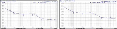
Figure 9: Relative to a 1GHz Signal | Relative to a 2GHz Signal
- Closed loop feedback
Not all Qubits are the same. Optimizing the control waveform to get the best performance from a Qubit may take several iterations of Control-Measure-Adjust-Control all in a very short time frame. Having the ability to digitize and process the signal in real time takes the experiment to the next level of performance.
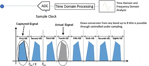
Figure 10: The optional Proteus Digitizer – can acquire signals up a maximum frequency of 9GHz
- Choose the best form factor.
Instruments come in many form factors and choosing the best form factor to meet the experiment needs is important. Understanding the capabilities of each form factor is key in this decision process. For experiments that require a lot of adjustments and alignments by the scientist an instrument with a front panel Graphical User interface (GUI) would be the best choice. If a front panel is not required as remote control for the primary interface, then an instrument without the screen may save some bench space and cost. However, it is important to consider ultimately how many channels the experiment will use and what data transfer rates are required. For channel counts higher than twelve or when fast data transfer rates are required a modular solution based on PXI offers the best performance as well as being an industry standard.

Figure 11: Proteus family of form factors